Google Sheets 101: A Beginner's Guide

Meghan Donovan Jan 26, 2020 3:00:00 AM

Microsoft first invented the Excel spreadsheet, and later Google offered their own version of .XLS, with Google Sheets.

Although Sheets are not difficult to use (like most Google products, this spreadsheet app is intuitive and very user-friendly), there might be a learning curve and there are a few tricks to getting the most out of the features available in Google Sheets.

With Google Sheets, you can create and edit spreadsheets directly in your web browser—no special software is required.

Multiple people can work simultaneously, you can see people’s changes as they make them, and every change is saved automatically.

Practice always makes perfect, and the goal is that by the end of this Sheets user guide you will have a grasp of beginner, intermediate, and advanced features, and you'll also know that you always have a reference to come back to should you fall into confusion.

Google Sheets 101 Table of Contents

What is Google Sheets?

google-sheets-1 Sheets is a free cloud-based spreadsheet app available from Google. Unlike previous spreadsheets where you had to download software, this opens in a normal webpage. You can do data analysis, or a simple spreadsheet for whatever you need.

What is the Difference Between Sheets and Excel?

Microsoft Excel was one of the originators online spreadsheet software. Although Sheets is similar to Excel, there are a few differences.

Google Sheets is cloud-based, and Excel is a downloadable desktop program. Sheets automatically saves on the cloud where everyone can access it.
Collaboration is actually within Sheets, whereas Excel does not have the proper functionality of this.
Both have charting tools and different types of Pivot Tables for data analysis.
Excel can handle larger datasets than Sheets, but Sheets still has a limit of 2 million cells.
Google Sheets works very well with all other Google Services and other online third party sites.
Both have scripting languages that extend their functionality and the ability to build custom tools.
Google Sheets uses Apps Script which is similar to Javascript, while Excel uses VBA.

Benefits of Google Sheets

The main benefits of Google Sheets are that it is free, collaborative and able to do a wide range of features. All teams can work on the same spreadsheet, at the same time, in real time. It is also extremely easy to use, while still being able to process complex data.

Creating Your First Google Sheet

First head here and click on “Go to Google Sheets,” in the center of the page.

You will then be prompted to log in. If you do not have a Google Account this would be the time when you should create one. After you have logged into the Sheets main page, you will see any of your previous spreadsheets, and options for spreadsheet templates. The first square will be a huge multi-colored plus button (+), and this will create a new blank Google Sheet.

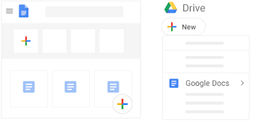
Opening Your First Sheet from Google Drive

You can also create sheets directly into your Google Drive. First head to your Google Drive, and simply click on the blue button entitled NEW. Then select Spreadsheets, and it will be created in your main drive folder. Here you can also create folders and organize your spreadsheets however you would like.

Editing Your Google Sheet

First you can rename your Sheet in the top left corner. It will automatically be named “Untitled spreadsheet.” Click on this and name it whatever you please.

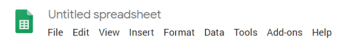
Your menus will be just below the name of your sheet, including functions such as: File, Edit, View, Insert, Format, Data, Tool, Add-ons and Help. Your columns are labeled A through Z and run horizontally across the page, while your rows are labeled by numbers 1- 1000.

Each cell is an intersection of a column and row. For example, column B and row 11 would be B11. Anytime you want to access this cell, it would be through utilizing the name B11.

Selecting, Entering, Moving & Deleting Data

In Google Sheets it is easy to select, enter, move, and delete data. Here's how:

Selecting: When clicking on any cell, you will notice a blue perimeter around the cell. This means you have selected this cell.
Entering: Clicking the cell once will highlight the entire cell, while clicking twice will actually enter the cell. When you start typing, you will automatically see your data entered in the cell.
Moving: When you hit enter, you will be moved down to the next cell. If you hit the tab key, you will move from one cell to the right rather than down. If you happen to be stuck in a cell, press escape which will deselect the contents and simply have the cell selected.
Deleting: Click the cell once, and hit delete to delete the entire contents of the cell. If you click twice you will see the cursor, so either select the data you would like to delete, or keep deleting until it is all gone.

Making Mistakes (Auto-Save Feature)

One amazing feature of Google Sheets when you're working with an internet connection is the constant auto-save feature. As you work your document will be automatically updated, saved, and synced to the Cloud so it's available from anywhere and you won't lose any of your work in the event of a computer crash or sudden loss of power.

If you happen to make a mistake at any time you can immediately press Cmd+Z (on a mac) or Ctrl+Z (on a PC). This will undo the previous step that you just completed. If you want to redo, you can press Cmd+Y (on a Mac), or Ctrl+Y (on a PC). You can also undo and redo using the arrows directly under the menu File and Edit.

Additionally, there is the option to view all the changes you, or anyone, has ever made to the spreadsheet. Simply click “All changes saved in drive,” at the top next to Help on the menu bar. This will take you to all versions of your sheet, which you can view and you can revert to a previous version should you wish to (but be careful, once you revert you will lose any data that has been entered since that version).

Columns And Rows

Changing the Size, Inserting, Hiding, Unhiding and Deleting

Selecting a row or column: Click the number (row) or letter (column) that you would like to select. This will highlight the entire row or column with a perimeter in blue.
Change the size of a column: The width of a column or height of a row can be changed by hovering your cursor over the grey line on the edge, until a line with an arrow pops up. Then click this, and drag the cursor whichever way you would like to grow or shrink the column or row.
Add additional columns or rows: First click on the column or row where you would like to insert a new one. Select this column or row, and right click for the options menu. For Columns, select either Insert Before or Insert After, for Rows select Insert Above or Insert Below. If you would like to add extra columns or rows at the end of your Google Sheet but have gotten to the 1000 mark do not worry. You can add up to 2 million cells which is 50,000 rows and 40 columns. You should realize that your sheet may slow down after 10,000-20,000 rows containing data or complex formulas.
Multiple Sheets: Adding, renaming and removing
Google Sheets has the option for multiple tabs within one Google Sheet. This is great for separating different data, or organizing Sheets according to different users. At the bottom of your sheet there will be a “+” button, and next to that 4 lines horizontally stacked, which is the index button.
Adding: Pressing the “+” button will allow you to add a sheet automatically.
Renaming: Clicking the small arrow next to the name of any sheet, will allow you to bring up the menu. You can then rename, delete, hide or unhide any sheets.
Removing: Similar to renaming, follow the same process and click delete.

Formatting

The formatting options for Google Sheets can be found on the top toolbar.

Here you can format such as make text bold, align text, or create currency. These are very similar to those found in Docs. To format a table with alternating row colors (also known as banding), simply select Format, then Alternating Colors. To remove all formatting from either one cell, or a range of cells press Cmd + \ (on a mac) or Ctrl + \ (on a PC).

Data and Basic Formulas

There are a few automatic formulas that occur in Sheets. The first are with dates. When inputting a date such as January 10 2019, it will automatically change it to 1/10/2019. All numbers, dates, percentages and currency will be automatically right aligned, while text will be immediately left aligned.

Math is automatically completed. For example, type (=), and then type your formula such as 4/2 (=4/2). You will see that the answer will automatically pop up with the option to X out.

Functions: Counting, Sums, and Averages

These formulas are a bit more complex, and very useful.

Counting: This will help you to count numeric values in a dataset. If you click on any cell, type (=) and then the word COUNT. A menu will pop up as soon as you type C and select COUNT. Next a window will pop up that shows different formula syntax and will help to guide you to fill it in. For example, if you wanted to count everything within B3 through B25 you would write =COUNT(B3:B25). For counting text you will have to use COUNTA instead.
Sums: This is a similar process, but instead of COUNT you will use SUM. Example =SUM(B3:B25)
Averages: Once again the process is the same, but instead it is =AVERAGE(B3:B25)

Functions vs. Formulas

Functions refer to a single word (COUNT), where formulas refer to everything after the equal sign ( =COUNT(B3:B25) ).

Unique Features & Google Sheets Techniques

There are a few features that are specific to Google Sheets as a cloud software, as compared to desktop software.

We'll cover those here, and also explain some beginner, intermediate, and advanced Google Sheets tips and techniques in this section.

Beginner Techniques

Comments and notes: There is the ability to add comments or notes without actually placing them in your sheet. You can also tag people with their email address if you would like them to see the comment. Then they can respond after they have read or fixed the issue. To add a comment to specific cell, select the cell, and right click. Select “insert comment” on the menu and fill in your comment. To tag someone type “+” plus the name or email that is in your contacts. Comments can be edited, deleted, linked, replied to and resolved (which will archive the comment). All comments will be reachable from the comments button on the top right of the screen.
Sharing: Although tagging someone in a comment is a form of sharing, you can also share an entire sheet with someone. This is great because you will be able to see any changes they make in real time. You have 3 options for sharing: View-only access, Comment-only access, and Editing access. View-only, allows the other person simply to view, Comment-only allows other people to make comments but no changes to the data in your sheet, and then Editing access allows full editing changes and access to the other people with whom you have shared your sheet. Sharing options are found by clicking the blue button in the top right corner.
Collaboration: After you have shared your sheet, the presence of anyone who has access will show up in two ways. The first way is with their cursor, meaning whatever has been selected. Additionally their presence will be visible at the top of the page.

Intermediate & Advanced Techniques

Freezing panes: This is helpful for when you have rows of data that go beyond one length of your screen. Let’s say your screen will show you as far as 28 rows. After scrolling past row 28 you will no longer be able to see the headings on the top of your screen. This can be difficult if you need to see the context of your columns. In order to see this you can freeze the heading rows. First select the row in which you would like to freeze up to, for example 5. Next click on View, then Freeze and select Up to current row (5).
Formulas across sheets: If you would like to link data between sheets, there is a specific way to go about this. For example, if you want to use a heading from cell A1 in Sheet 1 and place it into Sheet 2, then you will need to start with =Sheet1!A1 entered into A1 on Sheet 2. Again as an example, if you would like to place this as a sum into a different set of cells you would put =SUM(Sheet1!D4:D17).
Conditional formatting: This is a technique that allows you to apple different formats to certain cells, based on specific conditions. This might be used to color code certain numbers such a positive or negative growth. First you will need to obtain a plain copy of the membership table by hitting Cmd + Z (on a Mac), or Ctrl + Z (on a PC). Next you will need to highlight the final column, and select Format from the menu, and finally Conditional formatting. Here you will be able to apply this formatting to a range, style and other options.
Data sorting: If you need to sort your data such as, from highest to lowest, or greatest to least first highlight the entire table. Then, you will need to go to Data, and then Sort range. First select the “Data has header” option, and how you would like it to sort from A-Z or Z-A. This does not necessarily mean in alphabetical order, but rather A symbolizes highest, and Z symbolizes lowest. Therefore if you have a data set of 100, A will mean 100, and Z will mean 1.
Data filtering: After sorting, you may want to filter your data as well. Head to Data and then Filter. Next you will need to click on an icon that looks like an upside down triangle. It will not turn the table green and you will see three horizontal lines that make up an upside down triangle. You will click on this, and see a menu pop up, and here you can choose your settings. To remove a filter, click this button again, and under “Filter by conditions”, change the rule to None.
Adding charts: Highlight any single column and got to Insert, then Chart. This will create a default chart, as well as opens an editing tool in your sidebar. In this area you will have the option to change both the chart type and data range, as well as other customized formatting options.
Explore Feature: Google Sheets has an AI option, which allows your sheet to create charts or formulas for you. The feature that performs this is called Explore, and can be found in the bottom right corner. Essentially, simply select any part of your chart, and click Explore. Then you will receive AI insight on your selection.

Now It's Your Turn: Put Google Sheets to Work for You

Although Google Sheets can seem daunting at first, after a few days of using the system, you will find it to be much more simple than other desktop versions of spreadsheets. And all of your Sheets download exactly the same way as Excel files, which is very handy for working with desktop users and forwarding spreadsheets to clients who may be more comfortable with Excel.

Bookmark this guide as you get the hang of using Google Sheets, or review one of our favorite Google Sheets resources which we've included as links below. If you're new to relying on a modern spreadsheet app to organize your data ... welcome! You will soon realize how helpful Google Sheets can be, and the impact that powerful spreadsheets have made on businesses.

And if you're a business using G Suite (or considering switching to Google from Microsoft), contact Suitebriar.

We provide white-glove support and training tailored to the needs of your business to help you make the most of your investment in the cloud.

info@suitebriar.com

+1 888 545 3685