9 Google Sheets Formulas That Will Make You More Productive

Google Sheets is extremely powerful, with plenty of built-in functions that can help improve your productivity.

Unfortunately, many people use Sheets without fully leveraging all of its power. Today, we’re going to share 9 Google Sheets formulas that you absolutely must know and use. These powerful formulas can transform the way you work, and increase your productivity.

Ready? Let's dive in.

Stay Up-to-Date with the TODAY() Function

One of the most frustrating things that can happen to you is when you’ve spent a few hours on a spreadsheet, printed it out (or emailed it), only to find out that you didn’t update the date. Not only does that look unprofessional, but it can create havoc for an accounting department, marketing department, or (let's face it) any department.

To fix this, simply insert =TODAY() wherever you want the date to be inserted.

This Google Sheet formula will always display the current date, even if the last time it was opened was three months ago. This is especially important if you have multiple spreadsheets to update/print/email out regularly. One less thing to do!

Recommended: Google Sheets User Guide - Google Sheets 101

Use the COUNTIF() Function to Count Certain Values

The next function you can use to help you with your Google Sheets spreadsheets is the COUNTIF() function.

This powerful Google Sheet formula can be used to count numbers and even text. Here are two formula examples to look at:

• =COUNTIF(A2:A10,“>1.00”)
• =COUNTIF(A2:A10,"A")

Both of these formulas will count the cells in a given range if the criteria matches.

In the first example, any value greater than 1.00 will count as 1. However, it will not count the value, just the count of the number of cells that match this criterion.

In the second example, any value that is equivalent to an A will count as 1. This could be used by teachers to quickly count how many students scored an A on their last exam.

This can help to reduce your time spent counting all the cells that fit a certain criteria, even giving you the ability to track more metrics in your spreadsheets!

Take this example, in which a COUNTIF formula in Google Sheets is used to count the number of students with certain assessment scores:

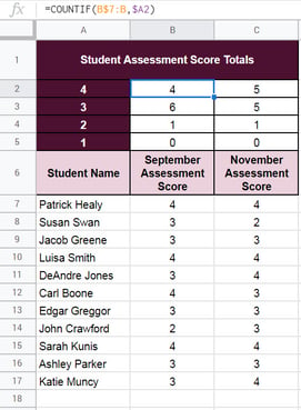
You can quickly see how in a large data-set, this powerful Sheets formula can provide a quick, top-level view of grade-level performance and trends to Principals and Administrators.

Use the SPLIT() Function to Separate Data

Here’s one that we’ve used plenty of times. The SPLIT() function is designed to split data from a single cell into multiple cells. If you have a long string value like the kind found in a .CSV file (Comma Separated Value), you can break it out for easier data manipulation. Below is an example of how split works.

As you can see, there is a long string of data in the A1 field. If you look at the formula in the C1 field, it says =SPLIT(“A1,”,”). Look at the value in the C1 field and the fields to the right of it. Now, they are all split wherever there's a comma, and all the commas have been removed.

You can use this for names, addresses, etc. And you can split data on any deliminator ... it doesn't have to be a comma (this can be good for separating day / month / year data from date text values so you can easily sort and filter your data.

Use CONCATENATE() to Put Multiple Strings Together

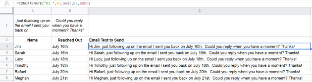
After splitting everything up using the =SPLIT() function, it’s time to put them all back together. This time we’ll use the CONCATENATE() formula to rejoin everything. Using the example above, we would type in =CONCATENATE(C1,",",D1,",",E1,",",F1,",",G1,",",H1,",",I1).

Now, if you noticed, we didn’t use =CONCATENATE(C1:I1); this would cause undesired results. Instead, we added a string delimiter between each cell (in this case we used a comma; you could use anything). This way, we reverted the string back into its original form.

This can be used to blend first and last names together, mailing addresses, and so much more. If you're in sales, you can even use this formula to generate follow-up email text in a manner similar to using merge tags in some high end CRMs (as in the example below).

Concatenate is a very powerful Google Sheet formula that you can use creatively in a number of ways. One of my favorites.

Use TRIM() to Remove Extra Spaces

Another function that you need to use more is the =TRIM() function. What this does is remove any excess spacing in your cell. Let's look at this sentence:

 “Jenny went to the store      to get some milk and eggs.       While she was out, she lost her purse and couldn’t get any milk.”

That sentence has a lot of dead space. Using the =TRIM() function, that sentence would be trimmed down to the following:

“Jenny went to the store to get some milk and eggs. While she was out, she lost her purse and couldn’t get any milk.”

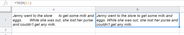
All of the dead space has been removed. The =TRIM() function will also remove extra whitespace from in front of the sentence and behind the sentence too.

This is useful when you are importing data that hasn’t been scanned/tested for purity, and can save you a lot of time when you need to clean up data that's poorly formatted.

Use TEXT() to Convert Numbers or Values to Another Format

Here is another function that you can’t live without. The =TEXT() function helps to make your data look uniform. Let’s look at the example below: 

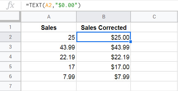
As you can see, the “A” column represents sales from some company. It looks like they made five sales for the day. However, some values are in decimal format and some are in whole number format. This can be difficult to look at when you are trying to manage accounting spreadsheets. To fix this, we’ve applied the formula in the “C” column and the result is shown in the “E” column.

Which one looks better to you?

Of course this is just one of the many ways you can use the TEXT() function. We'll leave it to you to get creative and put this one to use at your business.

Use LEFT() and RIGHT() to Extract Data from Long Strings

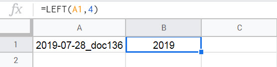
This is a great tool for gathering just the information you need from a string. Let’s say that you are looking at filenames. If the filename started with the date (format yyyy-mm-dd), you could use the =LEFT() function to easily extract the year by counting the number of characters from the left side of the filename that you wanted to extract (in this case four), like so:

The =RIGHT() function just starts from the back of the string and works to the front. So, if the date were at the end of the file, you could do the exact same thing using the =RIGHT() function instead.

Use GOOGLETRANSLATE() to Understand Another Language

Not all the data you work with will be in your native language. When this happens, you can convert the data using =GOOGLETRANSLATE(). This is a rather intriguing function as you can assign the primary language and the conversion language, or you can simply use "auto" and let Google Translate detect the source language that is to be translated:

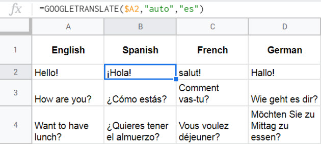
For instance, if you have the text "Hello Everyone!" in cell A5 in English but need it in French, you would use =GOOGLETRANSLATE(A5,"en","fr"); that would convert “Hello Everyone!” into “Bonjour à tous!” directly in the spreadsheet.

Recommended: Google Sheets vs Excel - Which Spreadsheet App is Best for You?

The Power of the IF() Function

This has to be the most commonly used function in Sheets. And if you aren’t using it, you are spinning your wheels.

This powerful formula can be used to quickly identify the highest profit customers in your database. If you'd like to quickly identify the customers that have made a purchase that resulted in a profit of more than $250, for example, you could use an IF formula like this, which flags those customers with a "YES" value:

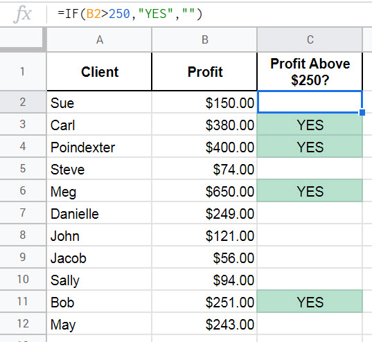
Sure, this a very basic way to use this function, but it's a good example of how you could use it in your business.

The =IF() function is probably one of the most used formulas in Google Sheets, and you can get even more advanced by using the IFS() function to qualify data in more than one way.

For example, let's take the student assessment score data example we used earlier in the article.

Let's say you are a school administrator using G Suite for Education.

You've tallied up the score totals quickly using a COUNTIF function, but now you want to quickly sort through the list of 2nd grade student assessment scores to identify students who may be falling behind and who may require extra support.

To do this, you could use the IFS formula in Google Sheets to identify the students whose assessment score went down from what they previously scored.

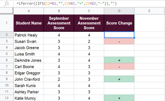
The formula above leaves column D blank if the score stayed the same, adds a "+" if the score went up, and a "-" if the score went down.

You can even add conditional formatting to flag every student whose scores went down in red, and every student whose scores went up in green, as I've done in the example above.

This short video shows you how you can set up conditional formatting to provide visual queues in Google Sheets:

This could save you time and energy, and would allow you to quickly put together a list of students to check-in on and potentially dedicate extra resources to.

And once you become a really advanced Sheets user, you can even sync your document with Gmail and set up automatic emails to the teachers whose students scores went down, asking if they feel that any of these students need extra resources. With Calendar, you can invite those teachers to quickly schedule a meeting to speak with you about what they feel are important next steps to address the needs of those students.

The possibilities are endless, especially if you leverage the power of Google Sheets as part of G Suite.

Start Using These Google Sheets Formulas Today

If you aren’t using these functions to build effective Google Sheets formulas, you should be. Once you get comfortable with them, your productivity will go up quickly. Even though the tasks seem menial, and you may not be working with a large data set today, these Sheets functions will make it possible to complete a task that could take an hour in under ten minutes.

What could you do with an extra fifty minutes of free time?

Probably a lot.