
Google Sheets is a spreadsheet application available for free or as part of the Google Workspace (formerly G Suite) productivity bundle. It offers full spreadsheet capabilities and provides amazing opportunity to work with text and numerical data. However, using Sheets requires a learning curve to unlock the true power of the app.
Data Validation is one ability every serious Google Sheets user should have in their arsenal of skills. That said, managing data in such a way is not inherently easy. More accurately, you’re not going to get started with data validation if you’ve never used a spreadsheet program before.
So, what should you do?
Well, reading this article is a good start because here you will find data validation examples and how to leverage them in Google Sheets. If you have a need for data validation, your reasons for reading on are evident. However, if you’re new to Sheets and just want to expand your skillset, why is data validation important?

When using data validation, your goal is to ensure the data in the spreadsheet is logical and correct. You may be thinking you can check this yourself, but that’s not so simple. Some spreadsheets include massive datasets so sifting for errors is time consuming and likely to end in error. Instead, you can validate the data.
Google Sheets makes this easy with its built-in Data Validation feature:
Google Sheets Data Validation with a Drop-down List
Drop-down lists are probably the most common form of data validation in Google Sheets. The app provides two ways to create a drop-down list:
- A list of items
- From a range
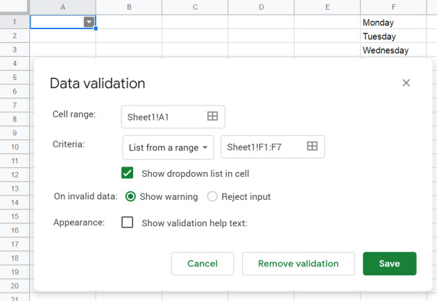
Let’s start with creating a drop-down menu using the “list from a range” method in Google Sheets. Below are the steps to create this simple menu:
- Step One - Open the sheet of the list you want to appear as the drop-down menu
- Step Two - Head to the menu bar at the top of the page, then Data > Data Validation
- Step Three - In the “Cell range” box, set to A1, choose the “Criteria” section select “List for a Range” and input your range. (Our example is F1:F7)
- Step Four - Click “Save”
There are some optional settings you can also use.
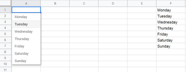
- Check the box next to “Show drop-down list in cell”. If you don’t select this option, no visible drop-down list will occur visible. However, clicking on the first cell (A1) will open the list.
- Where the option “On invalid data appears”, you can choose between “Reject input” and “Show Warning”.
Drop-Down List in Google Sheets with List of Items Method
There’s another way to create a drop-down list for Data Validation in Google Sheets. You now know how to create a list through the “List from a Range” tool, but what about the “List of Items” feature?
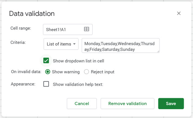
This is arguably more useful than creating a list by range. By using a list of items, the drop-down menu, you list individual items from your list in the Criteria section. Ensure the items are separated by commas:
- Open the sheet of the list you want to appear as the drop-down menu
- Head to the menu bar at the top of the page, then Data > Data Validation
- In the “Cell range” box, set to A1, choose the “Criteria” and section select “List of items” and input your list.
- Click “Save”
Less Common Data Validation Values in Google Sheets
When working with Data Validation in Google Sheets, arranging by range and list are not the only options. In fact, the app gives you several more options:
- Number
- Text
- Date
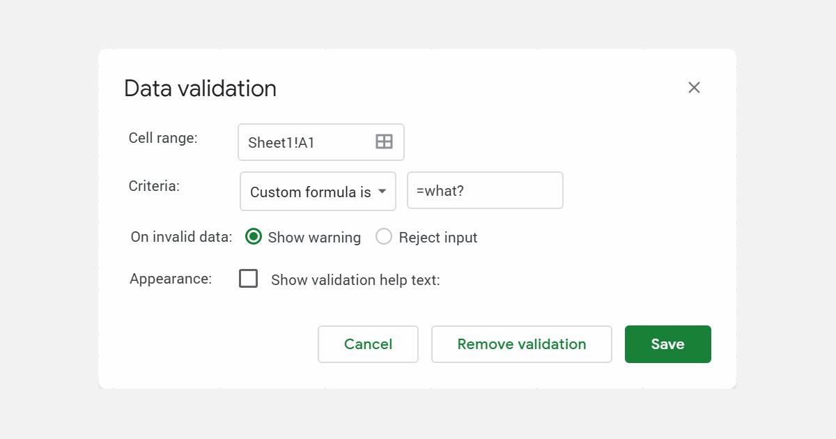
- Custom formula
- Tick box
Data Validation with a Tick Box
You can validate your Google Sheets data by organizing through Checkboxes (Tick Boxes). This ability is available in the “Criteria” section of the Data > Data Validation menu path.

Choosing this option changes the look and options in the Data Validation window. You will now see:
Cell range: This remains from the range and lists options and denotes the range of cells you want to include.
Use custom cell values: Tick boxes are clickable items in the spreadsheets, so you can both click and unclick them. If a box is checked, the corresponding cell value is either TRUE or FALSE. You can replace these values with your own custom value.
On invalid data - Show warning or Reject input: You can choose to only allow a mouse click to check or uncheck a box by selecting “Reject input”.
Number, Date, or Text Using Data Validation in Google Sheets
We’ve already spoken about the importance of data validation as a tool for ensuring all the data in your spreadsheets is accurate. Google Sheets Data Validation tool is extremely helpful, and for the most part you will be using the drop-down lists or tick boxes methods from above.
However, it is also possible to refine your data validation further and without much work. To do so, you can validate your information by looking at Text, Number, and Date.
Data Validation in Google Sheets by Numbers
Data constraints can also be set through numbers by changing the number in a range of cells or an individual cell. For the most part, the settings for doing this are uniform with the methods above, including heading to Data > Data Validation and changing the “Criteria” option to “Number”.
You will now be presented with the number data validation menu. Next to “Criteria” there is a drop-down menu with the following options:
- Between: Here you can enter the number between two preset numbers.
- Not between: This allows a set of 0 to 10 and you must enter a number larger than 10.
- Less than: With this option you can only enter a digit less than the preset (which is the number you will enter in the box).
- Less than or equal: Here you can enter a number less than or equal to the preset.
- Greater than: Only allows numbers that are greater than the preset.
- Greater than or equal: Limited to numbers equal to or greater than the chosen preset number.
- Equal to: You can only enter a digit that is the same as the preset.
- Not equal to: A number that is not the same as the preset.
Data Entry for Data Validation in Google Sheets

By using a date criteria for data validation, you can get more accurate formatted dates across a chosen range of your spreadsheets. Again, you’ll need to head to Data > Data Validation and then switch “Criteria” to “Date”.
Below are the settings you can work with:
A valid date: This setting checks the date value is current and not a text number.
The Criteria options also contain similar options to the “Number” criteria, such as before, on or before, equal to, after, on or after, between, not between.
Text Entry for Data Validation in Google Sheets
You can also set data validation or sort by text by heading to Data > Data Validation and setting “Criteria” to “Text”. Here you can choose the “Contains” option to search for specific words across your data.
Data Validation Made Easy in Google Sheets
And there it is.
You are now equipped with the ability to easily validate your data on Google Sheets.
While the concept of data validation may seem daunting at first, the above steps show that Google’s app makes it extremely easy to ensure your data is accurate across a spreadsheet.